Hyperparameter Tuning for Lead Scoring Models

Hyperparameter tuning can make or break your lead scoring model. It’s not just about the algorithm you choose - it’s about fine-tuning the settings that guide how your model learns. Here’s why this matters:

• Boost Performance: Even a 1% improvement in accuracy can lead to meaningful financial gains. For example, a tuned LightGBM model increased projected profit from $88,830 to $89,925.
• Avoid Pitfalls: Proper tuning helps prevent overfitting (too specific to training data) or underfitting (missing key patterns), ensuring reliable predictions.
• Key Parameters: Focus on impactful settings like learning rates, tree depth, and regularization strength. For Logistic Regression, tuning C and penalty type is critical. For tree-based models, parameters like max_depth and n_estimators make a big difference.

Tuning Methods:

• Grid Search: Tests all parameter combinations but is resource-intensive.
• Randomized Search: Samples parameter combinations, saving time.
• Bayesian Optimization: Uses past results to predict the best settings, ideal for complex models.
• Successive Halving: Quickly eliminates poor configurations by testing in stages.

Best Practices:

• Focus on impactful parameters first.
• Use metrics like ROC AUC, precision, and recall instead of just accuracy.
• Apply domain knowledge to set realistic ranges and avoid overfitting.

Hyperparameter tuning transforms lead scoring into a precise, data-driven process that helps sales teams prioritize high-value leads effectively.

Hyperparameter Tuning for Machine Learning: A Beginner's Guide

Key Hyperparameters in Lead Scoring Algorithms

Tuning hyperparameters is crucial for optimizing machine learning models used in lead scoring. Each algorithm comes with its own set of parameters that can significantly impact performance. Let’s dive into the key hyperparameters for three commonly used algorithms in lead scoring.

Logistic Regression

The most important parameter here is C (Inverse Regularization Strength). This controls the trade-off between fitting the training data and maintaining simplicity for better generalization. Smaller values of C enforce stronger regularization, reducing overfitting but possibly missing subtle patterns. Larger values allow for more complexity but can lead to overfitting noise in the data ^[7]. For example, using GridSearchCV to fine-tune this parameter has been shown to significantly improve logistic regression accuracy ^[7].

The penalty type also plays a major role. L1 (Lasso) penalty can shrink some coefficients to zero, effectively removing irrelevant features, while L2 (Ridge) penalty reduces coefficients without eliminating them entirely ^[7]. Additionally, the solver parameter determines how efficiently the model converges. For large datasets, saga or sag are preferred for faster processing, while liblinear works better for smaller datasets ^[7].

If the model struggles to converge (common in scikit-learn), increasing max_iter to 1,000 or more can resolve warnings ^[7]. Next, let’s explore hyperparameters for tree-based methods, which require a different approach.

Decision Trees and Random Forests

For decision trees, max_depth is a critical parameter. It limits the depth of the tree, balancing the ability to capture lead behavior without overfitting. Typically, an optimal depth falls between 4 and 10 ^[10]. Min_samples_split defines the minimum number of samples required to split a node, ensuring the model doesn’t create rules based on too few leads, which improves its ability to generalize ^[8].

Another key parameter, min_samples_leaf, ensures that each terminal node contains a minimum number of samples, reducing the risk of over-prioritizing outliers ^[8]. In Random Forests, n_estimators determines how many trees are built. While increasing this generally boosts accuracy and stability, it also raises computational costs ^[9][5]. Meanwhile, max_features introduces randomness by limiting the number of features considered at each split, which helps the model remain robust even with noisy or incomplete lead data ^[8][9].

"The performance of decision trees highly relies on the hyperparameters, selecting the optimal hyperparameter can significantly impact the model's accuracy, generalization ability, and robustness." - GeeksforGeeks ^[8]

Class imbalance is a common challenge in lead scoring datasets, where non-converters far outnumber converters. Parameters like min_weight_fraction_leaf and scale_pos_weight help ensure the model doesn’t skew toward the majority class ^[8][11]. For large datasets, tools like RandomizedSearchCV or HalvingRandomSearchCV can speed up the search for optimal hyperparameters ^[8][5].

Gradient Boosting Models

Gradient boosting models require careful tuning to balance complexity and performance. The learning rate (eta) works in tandem with n_estimators. A smaller learning rate improves generalization but requires more boosting rounds, which increases training time ^[14][15]. Instead of manually selecting the number of estimators, it’s often better to set n_estimators high and rely on early stopping to avoid overfitting when validation performance plateaus ^[12][14].

Max_depth controls how complex the trees can get and determines the level of interaction between lead features. While deeper trees can better fit the training data, they also risk overfitting. An optimal depth is usually between 4 and 10 ^[12][10]. Parameters like subsample and colsample_bytree introduce randomness by using only a subset of data or features for each tree, which helps prevent over-reliance on specific samples ^[11][13].

For imbalanced datasets, scale_pos_weight is particularly useful. It adjusts the weight of positive leads, improving the model’s ability to detect high-value leads in skewed datasets ^[11][13]. LightGBM, a popular gradient boosting framework, uses leaf-wise tree growth for faster convergence. However, this requires tuning parameters like num_leaves and min_data_in_leaf to avoid overfitting. For large datasets, setting min_data_in_leaf to higher values (hundreds or thousands) ensures the model doesn’t create overly specific rules that don’t generalize well ^[14].

Hyperparameter	Primary Role	Impact on Lead Scoring
learning_rate	Step size shrinkage	Smaller values improve accuracy but require more trees
n_estimators	Number of boosting rounds	Higher values capture more patterns but risk overfitting
max_depth	Tree complexity	Controls interaction level between lead features
subsample	Randomization	Prevents over-reliance on specific training samples
scale_pos_weight	Class balancing	Adjusts weights for positive leads in imbalanced datasets

Each algorithm has its own set of hyperparameters that can make or break its performance. Fine-tuning these settings ensures your lead scoring model is both accurate and reliable, regardless of the dataset’s challenges.

Techniques for Hyperparameter Tuning

Once you've identified the key hyperparameters for your lead scoring model, the next step is selecting a tuning method that can effectively enhance its performance. Below are some common techniques, each suited to different scenarios.

Grid Search

Grid Search is a methodical approach that tests every possible combination of predefined hyperparameter values ^[5]. For instance, if you're tuning a Logistic Regression model with three possible values for the regularization parameter C (0.1, 1.0, 10.0) and two penalty types (L1, L2), Grid Search will evaluate all six combinations. This thorough approach works well for models with only a few hyperparameters but becomes computationally expensive as the number of parameters increases ^[5].

Randomized Search

Unlike Grid Search, Randomized Search doesn't evaluate every combination. Instead, it randomly samples a set number of configurations from predefined distributions ^[16]. You control the process by setting a fixed number of iterations (n_iter), allowing for efficient exploration of the hyperparameter space ^[5]. This method is particularly useful for models with many parameters, like Random Forests, as it avoids the exponential time cost of exhaustive searches. It's especially effective for continuous parameters, such as learning rates, where distributions like loguniform can help explore a wide range of values ^[3].

Advanced Methods: Bayesian and Halving Grid Search

For scenarios where computational resources are limited or training is costly, advanced methods offer more efficient alternatives.

• Successive Halving: This technique operates like a tournament. All hyperparameter configurations are initially tested with minimal resources, such as a small subset of training data. Only the top-performing ones progress to the next round, where they receive more resources. This approach quickly eliminates weaker options, making it ideal for large datasets. For instance, if your lead scoring model processes millions of records, tools like HalvingRandomSearchCV can efficiently identify promising hyperparameter combinations ^[5].
• Bayesian Optimization: This method treats hyperparameter tuning as a regression problem, using past results to predict the most promising configurations ^[4]. It strikes a smart balance between exploring new possibilities and refining known good options. Bayesian Optimization is particularly effective for problems with fewer than 20 dimensions ^[17], making it an excellent choice when precision is critical, and training is resource-intensive. However, its sequential nature can limit parallel processing ^[3].

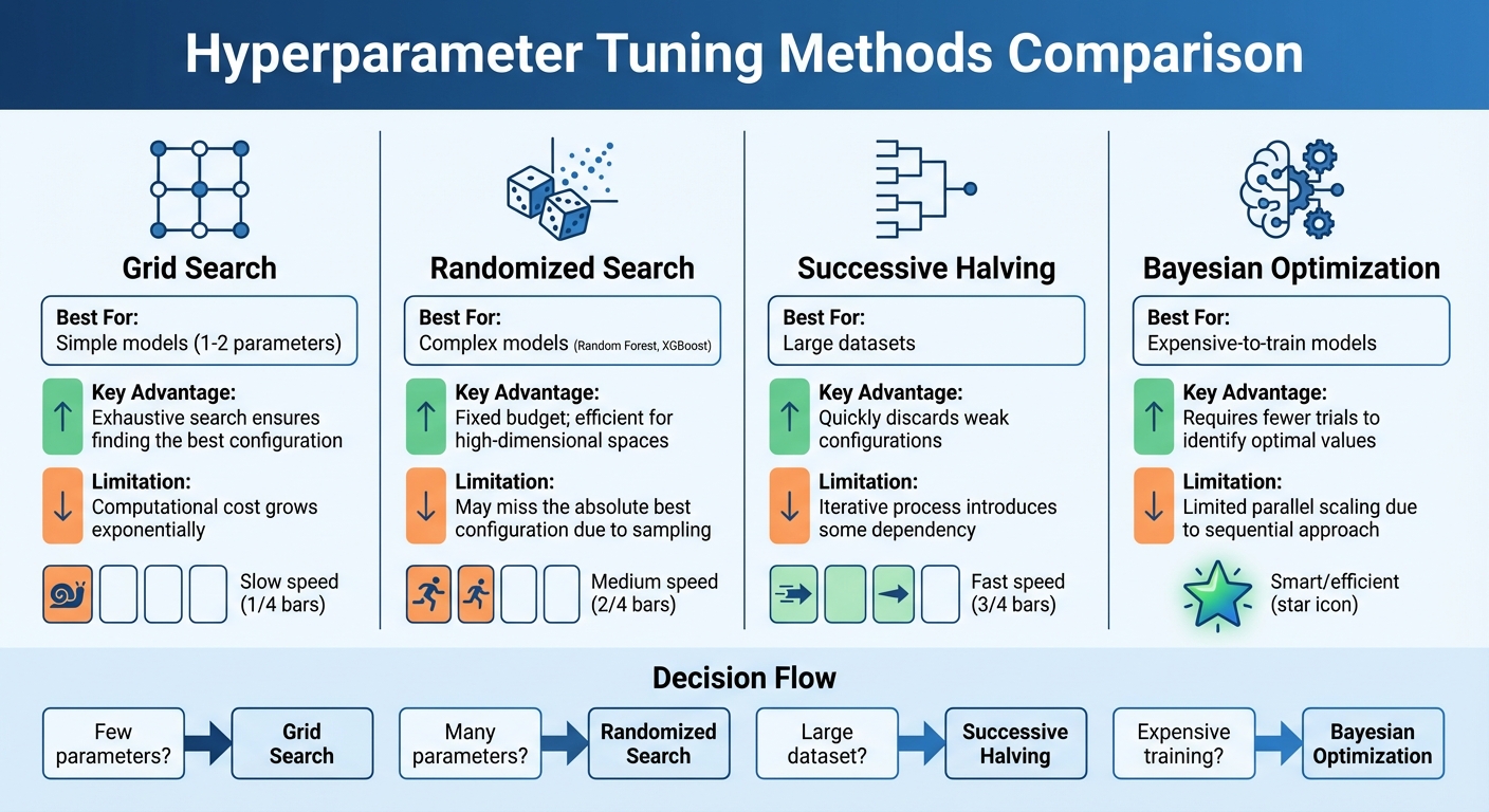
Technique	Best For	Key Advantage	Limitation
Grid Search	Simple models (1–2 parameters)	Exhaustive search ensures finding the best configuration	Computational cost grows exponentially
Randomized Search	Complex models (Random Forest, XGBoost)	Fixed budget; efficient for high-dimensional spaces	May miss the absolute best configuration due to sampling
Successive Halving	Large datasets	Quickly discards weak configurations	Iterative process introduces some dependency
Bayesian Optimization	Expensive-to-train models	Requires fewer trials to identify optimal values	Limited parallel scaling due to sequential approach

Up next, we'll dive into best practices for fine-tuning hyperparameters in lead scoring models.

sbb-itb-817c6a5

Best Practices for Hyperparameter Tuning in Lead Scoring

Building on the tuning techniques discussed earlier, these best practices can help fine-tune your model for better performance.

Start with the Most Impactful Parameters

Once you've identified the key hyperparameters, focus on the ones that have the greatest influence on your model's performance. Often, only a small number of parameters significantly impact the results, while others can remain at their default settings ^[5][3]. Think of hyperparameters as the critical dials on your model - small adjustments can lead to big changes.

For Logistic Regression, prioritize tuning C (regularization strength) and the penalty type (L1 or L2). These control overfitting and allow for automatic feature selection, especially when working with high-dimensional customer data. For tree-based models like Random Forest or Gradient Boosting, focus on parameters such as n_estimators, max_depth, and min_samples_leaf to strike a balance between model complexity and accuracy. With Gradient Boosting, the learning_rate is particularly important, as it influences the behavior of other parameters ^{[5][1][2][18]}.

The Google Deep Learning Tuning Playbook suggests classifying parameters into two groups: "scientific" (those that measure specific effects, like model depth) and "nuisance" (those that ensure fair comparisons, like learning rate) ^[18]. Start simple, and gradually increase complexity:

"The most effective way to maximize performance is to start with a simple configuration and incrementally add features and make improvements while building up insight into the problem" ^[18]

When exploring ranges for parameters like learning rates or regularization strengths, use a log-scale rather than a linear scale ^[3]. For instance, test learning rates at 0.001, 0.01, 0.1, and 1.0 instead of using linear steps like 0.1, 0.2, 0.3, and 0.4. This approach captures meaningful differences more effectively.

Use the Right Evaluation Metrics

Accuracy alone can be misleading in lead scoring. For example, if 95% of your leads don’t convert, a model that predicts "no conversion" for every lead would still achieve 95% accuracy - but it wouldn’t provide any value to your business ^[5][21]. That’s why more nuanced metrics are essential.

ROC AUC (Area Under the Receiver Operating Characteristic Curve) is a popular choice for lead scoring. It measures how well your model distinguishes between converted and non-converted leads across all probability thresholds, making it ideal for ranking leads by their likelihood to convert ^[21].

Other metrics to consider:

• Precision: This tells you how many of the leads your model identifies as high-value actually convert. It’s especially important when sales resources are limited.
• Recall: This measures the percentage of actual converters that your model correctly identifies. It’s vital when missing even a single potential lead could hurt revenue.
• F1-Score: This metric balances precision and recall, making it useful for datasets where non-conversions vastly outnumber conversions ^[21].

You can also create custom business metrics tailored to your goals. For instance, one case study optimized for profit by factoring in $120 revenue per conversion against a $15 cost for outreach. This approach led to a 1.2% increase in total profit ^[2]:

"The machine learning evaluation metrics you choose should reflect the business metrics you want to optimize with the machine learning solution" ^[20]

Metric	Business Alignment	When to Prioritize
ROC AUC	Lead Prioritization	Ranking leads by conversion likelihood
Precision	Sales Efficiency	When sales resources are limited
Recall	Revenue Maximization	When missing conversion-ready leads is costly
F1-Score	Balanced Performance	Avoiding bias toward precision or recall

The right metrics, combined with domain knowledge, can make your tuning process more effective.

Apply Domain Knowledge

Sales expertise plays a crucial role in defining realistic hyperparameter ranges, which can save computation time and improve your model’s generalization ^[3]. For example, understanding customer behavior can help you weigh the costs of misclassification. If sales resources are tight, prioritize precision. On the other hand, if missing even one qualified lead could result in a significant loss, focus on recall ^[2][19].

Tools like SHAP values can help ensure your hyperparameter choices don’t unintentionally introduce data leakage or overemphasize irrelevant patterns ^[2]. For instance, if historical data shows that leads who spend more than 20 minutes on your website have a 90% conversion rate, this insight can guide decisions about tree depth or feature interactions ^[2].

In a dataset with over 9,000 entries, applying domain knowledge to eliminate highly correlated economic indicators using Variance Inflation Factor (VIF) improved model interpretability without sacrificing performance ^[21]. This highlights how combining sales expertise with statistical techniques can lead to models that are not only accurate but also actionable for your team.

Implementing Hyperparameter Tuning with scikit-learn

Scikit-learn makes hyperparameter tuning straightforward with its built-in tools. To avoid errors caused by typos or incorrect parameter names, use estimator.get_params() to verify available parameters. When working on lead scoring, it's better to optimize for probabilities (e.g., scoring="roc_auc" or scoring="average_precision") instead of binary predictions, especially when dealing with imbalanced datasets.

For faster tuning, set n_jobs=-1 to utilize all available CPU cores and use error_score=0 to handle problematic parameter combinations without breaking the process. Always split your dataset into a development set for tuning and a separate evaluation set to test performance on unseen data. By default, scikit-learn retrains the best model on the entire dataset when refit=True is enabled.

Grid Search Example for Logistic Regression

When tuning Logistic Regression for lead scoring, focus on adjusting the regularization strength (C) and penalty type (l1 or l2). Here's an example of how to implement grid search for this purpose:

from sklearn.model_selection import GridSearchCV
from sklearn.linear_model import LogisticRegression
from sklearn.model_selection import RepeatedStratifiedKFold

# Define the parameter grid
param_grid = {
    'C': [0.001, 0.01, 0.1, 1.0, 10.0, 100.0],
    'penalty': ['l1', 'l2'],
    'solver': ['liblinear']  # Required for l1 penalty
}

# Set up the model
model = LogisticRegression(max_iter=1000, random_state=42)

# Configure cross-validation
cv = RepeatedStratifiedKFold(n_splits=5, n_repeats=3, random_state=42)

# Create the grid search
grid_search = GridSearchCV(
    estimator=model,
    param_grid=param_grid,
    scoring='roc_auc',
    cv=cv,
    n_jobs=-1,
    error_score=0
)

# Fit on your lead data
grid_search.fit(X_train, y_train)

# Access the best parameters and score
print(f"Best parameters: {grid_search.best_params_}")
print(f"Best ROC AUC: {grid_search.best_score_:.4f}")

The C parameter is tested on a logarithmic scale to identify meaningful differences across a wide range of values. For quicker tuning, consider using LogisticRegressionCV, which is optimized for calculating the regularization path.

Randomized Search Example for Decision Trees

When the parameter space is large, RandomizedSearchCV is a more efficient option compared to exhaustive grid search. It tests a fixed number of parameter combinations, making it ideal for models like Decision Trees. Here's an example:

from sklearn.model_selection import RandomizedSearchCV
from sklearn.tree import DecisionTreeClassifier
from scipy.stats import randint

# Define parameter distributions
param_distributions = {
    'max_depth': randint(3, 20),
    'min_samples_split': randint(2, 50),
    'min_samples_leaf': randint(1, 30),
    'class_weight': ['balanced', None]
}

# Set up the model
model = DecisionTreeClassifier(random_state=42)

# Create the randomized search
random_search = RandomizedSearchCV(
    estimator=model,
    param_distributions=param_distributions,
    n_iter=100,  # Number of parameter combinations to try
    scoring='roc_auc',
    cv=5,
    n_jobs=-1,
    random_state=42,
    error_score=0
)

# Fit on your lead data
random_search.fit(X_train, y_train)

# Get results
print(f"Best parameters: {random_search.best_params_}")
print(f"Best ROC AUC: {random_search.best_score_:.4f}")

The n_iter parameter controls how many combinations are tested, letting you balance thoroughness with time constraints. For even faster tuning on large datasets, try HalvingRandomSearchCV, which eliminates poor parameter combinations early in the process.

In a scikit-learn study, researchers used GridSearchCV with RepeatedStratifiedKFold (10 folds, 10 repeats) to compare SVC kernels. They observed that the 'rbf' kernel achieved a mean AUC of 0.9400, while the 'linear' kernel scored 0.9300 ^[22]. This highlights how systematic tuning can uncover meaningful differences in model performance.

Once you've fine-tuned your model with Randomized Search, you can integrate it into your lead scoring workflow for improved results.

Using SalesMind AI for Advanced Lead Scoring

After tuning your model, integrate it into your sales process for better lead prioritization. SalesMind AI can seamlessly incorporate your optimized model, leveraging it to rank prospects based on their likelihood of conversion. With features like an AI-powered unified inbox and automated follow-ups, SalesMind AI ensures high-priority leads get immediate attention, while others are guided through nurturing sequences. This combination of precise tuning and advanced automation can significantly boost your outreach efficiency.

Conclusion

Key Takeaways

Hyperparameter tuning takes lead scoring from being a guessing game to a data-driven process. With the right configurations, your model can more accurately identify high-value prospects, leading to better sales efficiency and increased revenue. Start with straightforward setups and prioritize the parameters that matter most - like regularization strength for Logistic Regression or tree depth for ensemble models. Metrics such as ROC AUC or average precision work best, especially when your dataset is imbalanced and most leads don’t convert.

For small parameter spaces, Grid Search is a dependable choice. Random Search, on the other hand, delivers comparable results while requiring fewer computational resources. If you’re ready for more advanced techniques, Bayesian Optimization offers an intelligent way to explore parameters by learning from past trials. Using conservative early stopping policies, like Median Stopping, can cut computational costs by 25%-35% without compromising model quality ^[6]. Importantly, aligning your tuning strategy with business goals - such as optimizing for a custom profit metric rather than standard AUC - can make a tangible difference. For example, one case study showed profits increasing from $88,830 to $89,925 by adopting this approach ^[2].

These strategies provide a clear path to putting hyperparameter tuning into action.

Next Steps

With these takeaways in mind, it’s time to refine and implement your lead scoring model. Begin by auditing your current setup to identify which hyperparameters have the most influence on your dataset. From there, establish a systematic tuning process using tools like scikit-learn. Keep an eye on training and validation curves to catch overfitting early, and always validate your final model on a separate evaluation set to ensure it performs well with new leads.

To make the most of your tuned model, SalesMind AI offers tools to streamline the process. It automatically prioritizes leads based on their likelihood to convert, initiates personalized outreach sequences, and instantly routes high-scoring prospects to your sales team. This combination of fine-tuned modeling and smart automation ensures your top leads get immediate attention, while your team can focus on closing deals instead of sorting through unqualified prospects.

FAQs

How does hyperparameter tuning improve the accuracy of lead scoring models?

Hyperparameter tuning is a key step in improving the precision of lead scoring models. Adjusting parameters such as learning rate, regularization strength, or tree depth helps the model identify patterns in the data more effectively, resulting in predictions that are far more dependable.

When a lead scoring model is fine-tuned properly, it assigns scores that align closely with a prospect’s true chances of converting. This enables businesses to focus on high-potential leads, ultimately streamlining sales efforts and boosting results.

What’s the difference between Grid Search and Bayesian Optimization for hyperparameter tuning?

Grid Search works by systematically testing every possible combination of specified hyperparameters within a given range. This method guarantees that the best configuration within the grid will be found. However, it can become quite resource-intensive, especially when you’re working with a large number of parameters or extensive datasets.

In contrast, Bayesian Optimization takes a smarter approach. It uses a probabilistic model to predict how different hyperparameter combinations will perform. By focusing on the most promising areas, it can identify optimal configurations more efficiently. This makes it a great choice for scenarios involving high-dimensional data or limited computational resources. That said, it does come with some additional computational overhead to maintain the model and can be sensitive to the chosen optimization strategy.

To put it simply, Grid Search is a straightforward option for smaller problems, while Bayesian Optimization shines in tackling more complex or large-scale tuning challenges where efficiency matters.

Why is ROC AUC a better metric than accuracy for evaluating lead scoring models?

When it comes to evaluating lead scoring models, ROC AUC often outshines accuracy, especially because lead-scoring datasets tend to be imbalanced. In these scenarios, accuracy might look impressive on the surface but can be misleading - failing to reflect the model's ability to pinpoint valuable leads.

What sets ROC AUC apart is its ability to assess how well the model differentiates between positive and negative leads across every possible decision threshold. This makes it a much more reliable metric for understanding how effectively the model ranks and prioritizes high-quality leads.